DETAILED INTRODUCTION -GGPLOT2

Detailed Introduction

                                                       DETAILED INTRODUCTION

About the ggplot2 Package

Introduction "ggplot2 is an R package for producing statistical, or data, graphics, but it is unlike most other graphics packages because it has a deep underlying grammar. This grammar, based on the Grammar of Graphics (Wilkinson, 2005), is composed of a set of independent components that can be composed in many different ways. [..] Plots can be built up iteratively and edited later. A carefuly chosen set of defaults means that most of the time you can produce a publication-quality graphic in seconds, but if you do have speical formatting requirements, a comprehensive theming system makes it easy to do what you want. [..] ggplot2 is designed to work in a layered fashion, starting with a layer showing the raw data then adding layers of annotation and statistical summaries.
 ggplot2,

First We look into the header of Diamonds and Mtcars data

head(diamonds)
head(mtcars)


         

        Comparison qplot vs ggplot
           qplot histogram
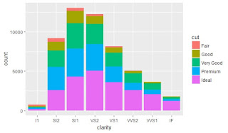
           qplot(clarity, data=diamonds, fill=cut, geom="bar")

                                          ggplot histogram -> same output
                                  ggplot(diamonds, aes(clarity, fill=cut)) + geom_bar()

Scatterplot

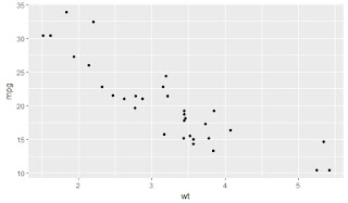
qplot(wt, mpg, data=mtcars)

Transform input data with functions

qplot(log(wt), mpg - 10, data=mtcars)

    Add aesthetic mapping (hint: how does mapping work)

qplot(wt, mpg, data=mtcars, color=qsec)

                        Change size of points (hint: color/colour, hint: set aesthetic/mapping)

                        qplot(wt, mpg, data=mtcars, color=qsec, size=3)

                        qplot(wt, mpg, data=mtcars, colour=qsec, size=I(3))

                                                          Use alpha blending

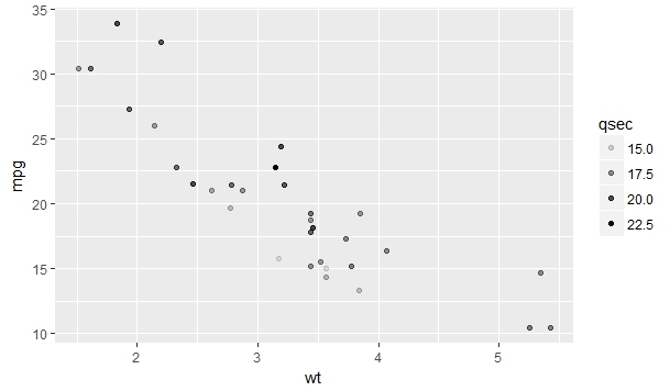
                                       qplot(wt, mpg, data=mtcars, alpha=qsec)

                          Continuous scale vs. discrete scale

                            head(mtcars)

                           qplot(wt, mpg, data=mtcars, colour=cyl)

                            levels(mtcars$cyl)

                           qplot(wt, mpg, data=mtcars, colour=factor(cyl))

                   Continuous scale vs. Discrete scale

                    head(mtcars)

                    qplot(wt, mpg, data=mtcars, colour=cyl)

                    levels(mtcars$cyl)

                   qplot(wt, mpg, data=mtcars, colour=factor(cyl))

              Use different aesthetic mappings

             qplot(wt, mpg, data=mtcars, shape=factor(cyl))

             qplot(wt, mpg, data=mtcars, size=qsec)

       Combine mappings (hint: hollow points, geom-concept, legend combination)

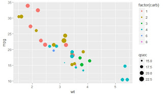
       qplot(wt, mpg, data=mtcars, size=qsec, color=factor(carb))

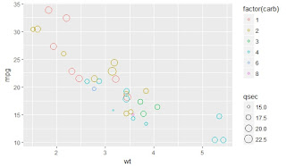
       qplot(wt, mpg, data=mtcars, size=qsec, color=factor(carb), shape=I(1))

       qplot(wt, mpg, data=mtcars, size=qsec, shape=factor(cyl), geom="point")

       qplot(wt, mpg, data=mtcars, size=factor(cyl), geom="point")

 Bar-plot

qplot(factor(cyl), data=mtcars, geom="bar")

Flip plot by 90°

qplot(factor(cyl), data=mtcars, geom="bar") + coord_flip()

 Difference between fill/color bars

qplot(factor(cyl), data=mtcars, geom="bar", fill=factor(cyl))

qplot(factor(cyl), data=mtcars, geom="bar", colour=factor(cyl))

Fill by variable

qplot(factor(cyl), data=mtcars, geom="bar", fill=factor(gear))

Use different display of bars (stacked, dodged, identity)

head(diamonds)

qplot(clarity, data=diamonds, geom="bar", fill=cut, position="stack")

qplot(clarity, data=diamonds, geom="bar", fill=cut, position="dodge")

qplot(clarity, data=diamonds, geom="bar", fill=cut, position="fill")

qplot(clarity, data=diamonds, geom="bar", fill=cut, position="identity")

qplot(clarity, data=diamonds, geom="freqpoly", group=cut, colour=cut, position="identity")

qplot(clarity, data=diamonds, geom="freqpoly", group=cut, colour=cut, position="stack")